Finally, some cleaning’s done on my very first Jupyter notebooks created between 2018-2019. Back then, I wasn’t capable of coding from scratch, so it was a process of literally copying & pasting chunks of code from the internet and running the woven code by hit-or-miss. Now that I became more proficient in Python, it was time to do some pruning and organization on these notebooks.

Why programming?

1. Data size The data I used to deal with were time-series of neural signals (either electrical outputs or fluorescent images) recorded over varying time lengths (minutes to hours) and its size would easily take up to GBs. Excel was just not enough to deal with these data and also very error-prone(due to dragging and modifying tens of thousands of rows at the same time).

2. Integrated data processing To analyze this kind of experimental data, multiple software (and machines) were needed at different stages of the work (collection, retrieval, analysis and visualization). A machine at the imaging facility had the software for data acquisition, a machine at the lab had the licensed software for data retrieval, and then my laptop served for analysis and visualization. Having limited access to the licensed software for analysis was another issue. I wanted an integrated solution for data retrieval, processing, statistic analysis and visualization.
   

Why Python?

Although I was advised to learn Matlab since it is the most abundantly used language in neuroscience laboratories, I didn’t like the fact that you still need a license for its usage which I couldn’t afford to. In the end, I chose Python over R only because it seemed to be the most widely used language in data sciences.

Results (examples)

For both types of data (images and electrophysiology recordings), the raw files (.CSV) were imported as a pandas dataframe and plotted by time.

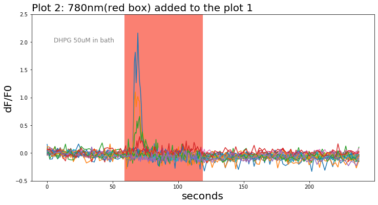
For live-cell imaging data, fluorescence changes (dF = F-F0) at each time point relative to the first X frames of each series (F0) were calculated as (F-F0)/F0 and plotted. Each line in the below figure indicates single-cell response and the red box indicates the duration of 780nm light stimulation applied to the tissue sample.

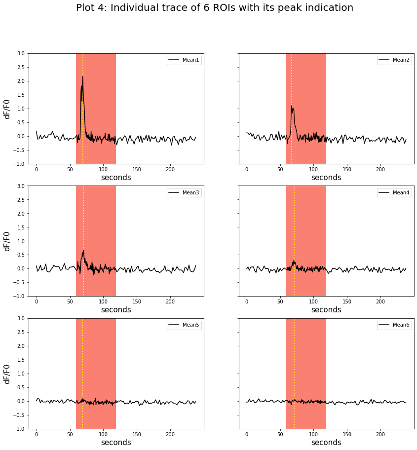
Local peaks(yellow dotted line) during the light stimulation from each trace were looked up from single traces. The time of appearance of each peak was found and noted.

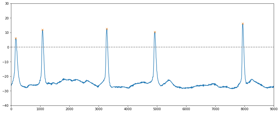
For electrophysiology data, local peaks were detected (orange X marks) by using the find_peaks module from scipy library.

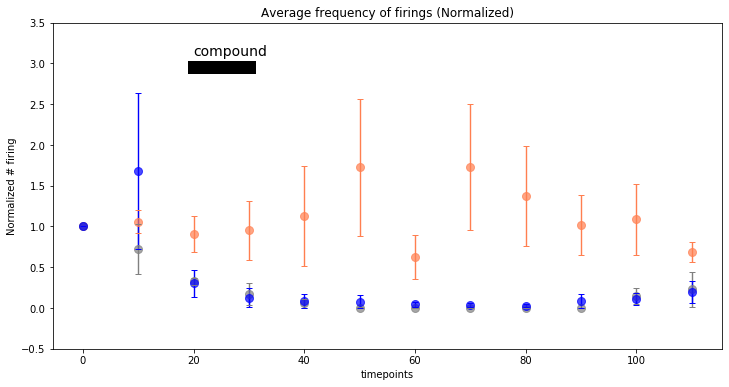
After the peak detection, the results were quantified for a comparison.

Impact

Using these codes, the time I put into the preliminary analysis was reduced from days to minutes. I could understand the results of the day in real-time and plan the next experiment based on it.